From Geometry to Gradient Descent: Harnessing Hypocycloids in Neural Network Optimization
Introduction:
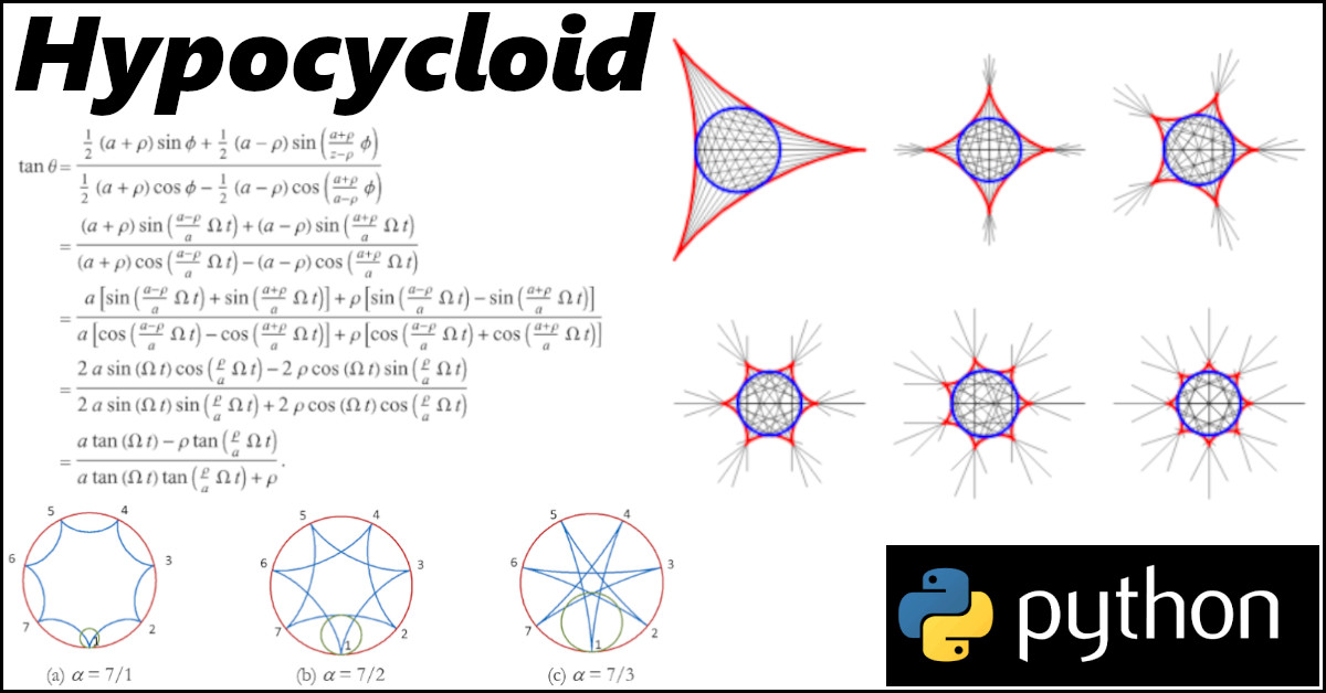
Optimization lies at the heart of machine learning, where algorithms iteratively adjust model parameters to minimize a loss function. Traditional gradient-based optimizers like Stochastic Gradient Descent (SGD) have been widely used, but recent innovations explore novel techniques to improve convergence speed and accuracy. One such innovative approach is the Hypocycloid Optimizer, which leverages the geometric properties of hypocycloids—a curve traced by a point on a smaller circle rolling inside a larger circle—to dictate the learning rate during training. This article dives deep into the theory, implementation, and experimental results of this unique optimizer.
Theoretical Background: Understanding Hypocycloids
A hypocycloid is a type of curve generated by a point on the circumference of a smaller circle as it rolls inside a larger fixed circle. The mathematical beauty of hypocycloids lies in their parametric equations:
Where:
- 𝑅 represents the radius of the larger fixed circle.
- 𝑟 is the radius of the smaller rolling circle.
- 𝜃 is the parameter, typically an angle that varies over time.
The Hypocycloid Optimizer: Implementation and Working:
The Hypocycloid Optimizer uses the geometric properties of hypocycloids to modulate the learning rate during training. Here's the implementation in Python using PyTorch:
import torch

# Hypocycloid-based gradient descent optimizer
class HypocycloidOptimizer(torch.optim.Optimizer):
    def __init__(self, params, lr=0.1, R=1, r=0.1):
        defaults = dict(lr=lr, R=R, r=r, theta=0.01)
        super(HypocycloidOptimizer, self).__init__(params, defaults)

    def step(self, closure=None):
        loss = None
        if closure is not None:
            loss = closure()

        for group in self.param_groups:
            R = group['R']
            r = group['r']
            theta = group['theta']
            lr = group['lr']

            hypocycloid_lr = lr * torch.cos(torch.tensor((R - r) / r * theta))

            for p in group['params']:
                if p.grad is None:
                    continue
                d_p = p.grad.data
                p.data.add_(d_p, alpha=-hypocycloid_lr)

            group['theta'] += 0.1  # Update theta for next step

        return loss
- Learning Rate Modulation: The optimizer adjusts the learning rate dynamically based on the cosine of the angle 𝜃, which evolves according to the hypocycloid formula.
- Parameter Update: The optimizer updates the model parameters using the adjusted learning rate, offering a unique trajectory for gradient descent.
Comparative Analysis: Hypocycloid Optimizer vs. SGD
To assess the effectiveness of the Hypocycloid Optimizer, we compared it with traditional Stochastic Gradient Descent (SGD). The experiments were conducted on a simple neural network, and the loss was tracked over multiple epochs.
import torch
import torch.nn as nn
import torch.optim as optim
from HypocycloidOptimizer import HypocycloidOptimizer
import matplotlib.pyplot as plt
# Define a simple model
model = nn.Linear(10, 1).cuda()
criterion = nn.MSELoss()
# Define hyperparameters
learning_rates = [0.1]
R_values = [1]
r_values = [0.1]
# Store loss values for comparison
sgd_losses = []
hypocycloid_losses = []
def train_model(optimizer_name, lr, R=None, r=None):
model = nn.Linear(10, 1).cuda()
criterion = nn.MSELoss()
if optimizer_name == 'SGD':
optimizer = optim.SGD(model.parameters(), lr=lr)
elif optimizer_name == 'Hypocycloid':
optimizer = HypocycloidOptimizer(model.parameters(), lr=lr, R=R, r=r)
losses = []
for epoch in range(100): # Increase epochs for better comparison
inputs = torch.randn(64, 10).cuda()
targets = torch.randn(64, 1).cuda()
optimizer.zero_grad()
outputs = model(inputs)
loss = criterion(outputs, targets)
loss.backward()
optimizer.step()
losses.append(loss.item())
if epoch % 10 == 0:
print(f'{optimizer_name} Epoch {epoch+1}/100, Loss: {loss.item()}')
return losses
# Train with SGD
for lr in learning_rates:
sgd_losses.append(train_model('SGD', lr))
# Train with HypocycloidOptimizer
for lr, R, r in zip(learning_rates, R_values, r_values):
hypocycloid_losses.append(train_model('Hypocycloid', lr, R, r))
# Plotting the results
plt.figure(figsize=(12, 6))
# Plot SGD losses
for i, losses in enumerate(sgd_losses):
plt.plot(losses, label=f'SGD (lr={learning_rates[i]})')
# Plot HypocycloidOptimizer losses
for i, losses in enumerate(hypocycloid_losses):
plt.plot(losses, label=f'HypocycloidOptimizer (lr={learning_rates[i]}, R={R_values[i]}, r={r_values[i]})')
plt.xlabel('Epoch')
plt.ylabel('Loss')
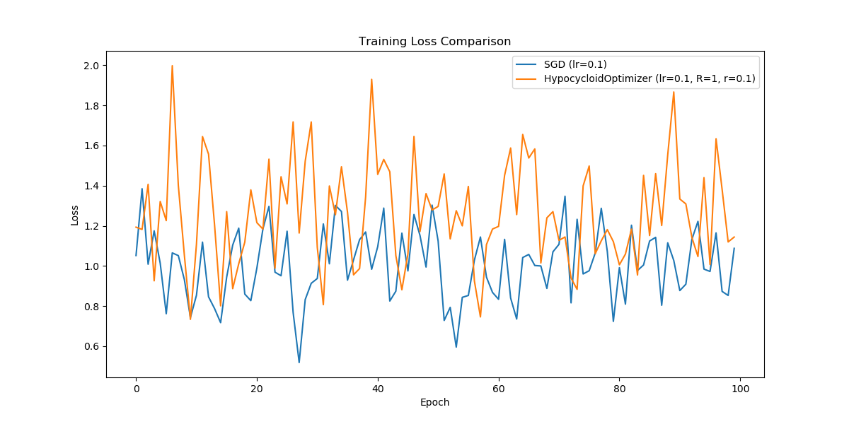
plt.title('Training Loss Comparison')
plt.legend()
plt.show()
The loss curves generated by the Hypocycloid Optimizer and SGD reveal fascinating insights:
- Spiky Behavior: The Hypocycloid Optimizer exhibits a slightly spikier loss curve due to the fluctuating learning rate, which may help escape local minima.
- Convergence: Both optimizers converged to similar loss values, but the Hypocycloid Optimizer's dynamic learning rate offers potential advantages in more complex scenarios.
Hyperparameter Tuning for Hypocycloid Optimizer
Hyperparameter tuning plays a critical role in maximizing the optimizer's performance. A strategy to fine-tune the parameters 𝑅, 𝑟, and learning rate 𝑙𝑟 is crucial. Here's a suggested approach:
import torch
import torch.nn as nn
import torch.optim as optim
import numpy as np
from itertools import product
from HypocycloidOptimizer import HypocycloidOptimizer  # Import the optimizer class

# Define the model
model = nn.Linear(10, 1).cuda()
criterion = nn.MSELoss()

# Define hyperparameter ranges
learning_rates = [0.001, 0.01, 0.1]
R_values = [0.5, 1, 1.5]
r_values = [0.1, 0.5, 1]
theta_steps = [0.01, 0.1, 0.5]

# Grid search
best_loss = float('inf')
best_params = None

for lr, R, r, theta_step in product(learning_rates, R_values, r_values, theta_steps):
    optimizer = HypocycloidOptimizer(model.parameters(), lr=lr, R=R, r=r)

    # Training loop
    for epoch in range(1000):  # Use a smaller number of epochs for hyperparameter tuning
        inputs = torch.randn(64, 10).cuda()
        targets = torch.randn(64, 1).cuda()

        optimizer.zero_grad()
        outputs = model(inputs)
        loss = criterion(outputs, targets)
        loss.backward()
        optimizer.step()

        if epoch % 1 == 0:
            print(f'Epoch {epoch+1}/10, Loss: {loss.item()}')

    # Evaluate on validation set (if available)
    # validation_loss = ...

    if loss.item() < best_loss:
        best_loss = loss.item()
        best_params = (lr, R, r, theta_step)

print(f'Best Parameters: lr={best_params[0]}, R={best_params[1]}, r={best_params[2]}, theta_step={best_params[3]}')
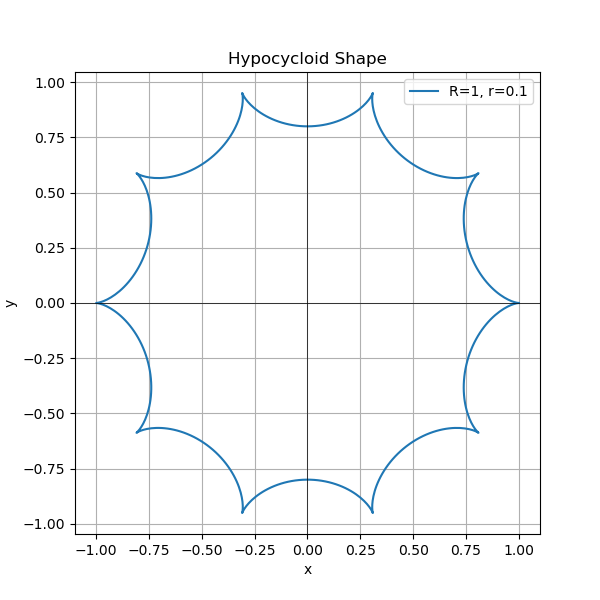
Visualizing Hypocycloids: Experimenting with Different Parameters
The geometric nature of hypocycloids allows for fascinating visual exploration. By plotting the hypocycloid curve for different parameters, you can gain intuition about how the optimizer's behavior is shaped.
import torch
import matplotlib.pyplot as plt
import numpy as np

R = 1
r = 0.1
theta_step = 0.01

# Function to calculate hypocycloid coordinates
def calculate_hypocycloid(R, r, theta_values):
    x_values = (R - r) * np.cos(theta_values) + r * np.cos((R - r) / r * theta_values)
    y_values = (R - r) * np.sin(theta_values) - r * np.sin((R - r) / r * theta_values)
    return x_values, y_values

# Generate theta values
theta_values = np.arange(0, 2 * np.pi, theta_step)

# Calculate hypocycloid coordinates
x_values, y_values = calculate_hypocycloid(R, r, theta_values)

# Plot the hypocycloid
plt.figure(figsize=(6, 6))
plt.plot(x_values, y_values, label=f'R={R}, r={r}')
plt.title('Hypocycloid Shape')
plt.xlabel('x')
plt.ylabel('y')
plt.axhline(0, color='black',linewidth=0.5)
plt.axvline(0, color='black',linewidth=0.5)
plt.grid(True)
plt.legend()
plt.show()
Conclusion:
The Hypocycloid Optimizer introduces an innovative approach to gradient descent by leveraging geometric properties to modulate learning rates. Through experimentation, comparison with traditional optimizers, and hyperparameter tuning, this article showcases the potential of hypocycloids in machine learning optimization. While the results are promising, further research and experimentation could unveil even more sophisticated uses of this fascinating geometric concept. By understanding and experimenting with hypocycloids, researchers and practitioners can explore new avenues in optimization, potentially leading to more efficient and robust machine learning models.